Week 5 Lecture: Introduction to Species Distribution Modelling (SDM)
week_5_lecture.RmdWhat are SDMs
- Sometimes called Environmental Niche Models (ENMs, I prefer SDM)
- Possible the most well-developed application of classic Data Science and Machine Learning (ML) in Biology
- They take in data on the environment at different sites or parts of a landscape and try predict where (or when, or how many) organisms will occur there. Data on the species themselves can also be used
- Traditionally done on single species at a time, but ‘joint’ species distribution models are increasingly common
SDMs as Data Science
- To make an SDM you use a Data Science workflow
- The final model used to predict species occurrence is fit using Machine Learning techniques
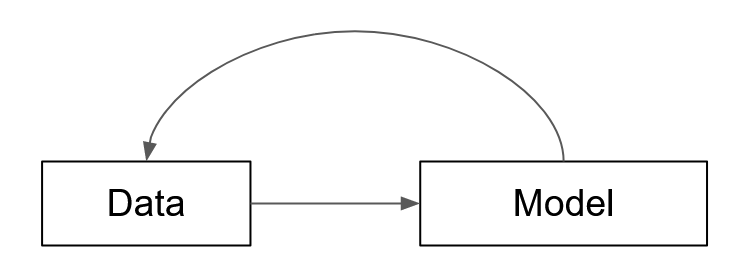
- A Data Science workflow has two major components:
- Data
- a Model
Data and Models
Data Processing Steps
Model Building
Data feeds into Models
Models inform Data processing steps
Data Science Steps
- A Question
- Collect Data
- Munge / Clean Data
- Transform Data for Model
- Analyze Data using Model
- Tune Model
- Validate / Test Model
- Interpret Model
Data Science Steps
- A Question
- Collect Data
- Munge / Clean Data
- Transform Data for Model
- Analyze Data using Model
- Tune Model
- Validate / Test Model
- Interpret Model
- We have covered some of this already
- We will cover the rest in the next 4 weeks
What is a Model?
- Encodes a relationship between a set of inputs and outputs
- For an SDM this is a (potentially complex and nonlinear) function that takes environmental variables as input and its output is an occurrence pattern (could be abundance, probability, suitability, etc.)
- Different Models differ in their assumptions, or ‘inductive biases’, and their parameters
- Models are ‘fit’ to data
- Parameters are chosen based on how well the Model’s output matches the real data
- This is an optimization problem
Fit a Linear Model to Reef Fish Data
- Base R has a good collection of statistical methods including the linear model.
-
RF_abundhas data on the abundance of different reef species at different reefs around the world
data("RF_abund")
RF_abund
## # A tibble: 781,983 × 25
## SpeciesName SiteC…¹ Abund…² Sampl…³ MeanT…⁴ MinTe…⁵ MaxTe…⁶ SDTem…⁷ ECOre…⁸
## <chr> <chr> <dbl> <dbl> <dbl> <dbl> <dbl> <dbl> <fct>
## 1 Abudefduf be… ACEH1 0 476 29.0 28.1 30.0 0.587 Wester…
## 2 Abudefduf be… ACEH10 0 476 29.1 28.1 30.1 0.602 Wester…
## 3 Abudefduf be… ACEH11 0 476 29.0 28.1 30.0 0.587 Wester…
## 4 Abudefduf be… ACEH12 0 476 29.0 28.1 30.0 0.587 Wester…
## 5 Abudefduf be… ACEH13 0 476 29.0 28.1 29.9 0.522 Wester…
## 6 Abudefduf be… ACEH14 0 476 29.0 28.2 30.0 0.526 Wester…
## 7 Abudefduf be… ACEH15 0 476 29.1 28.1 30.0 0.580 Wester…
## 8 Abudefduf be… ACEH16 0 476 29.0 28.1 30.0 0.587 Wester…
## 9 Abudefduf be… ACEH17 0 476 29.0 28.1 30.0 0.587 Wester…
## 10 Abudefduf be… ACEH18 0 476 29.1 28.1 30.1 0.581 Wester…
## # … with 781,973 more rows, 16 more variables: Presence <dbl>, OLRE <fct>,
## # MaxAbundance <dbl>, N_Obs <int>, Confidence_NObs <dbl>, T_Range_Obs <dbl>,
## # Confidence_TRange_Obs <dbl>, N_Absences_T_Upper <int>,
## # N_Absences_T_Lower <int>, Confidence_Occ_Tupper <dbl>,
## # Confidence_Occ_Tlower <dbl>, T_Upper_Absences <dbl>,
## # T_Lower_Absences <dbl>, T_Mean_Absences <dbl>, NEOLI <dbl>,
## # Depth_Site <dbl>, and abbreviated variable names ¹SiteCode, …Fit a Linear Model to Reef Fish Data
- First let’s choose a fish species to model
- Thalassoma pavo: Ornate Wrasse
knitr::include_graphics("images/week_5_lecture_insertimage_2.png")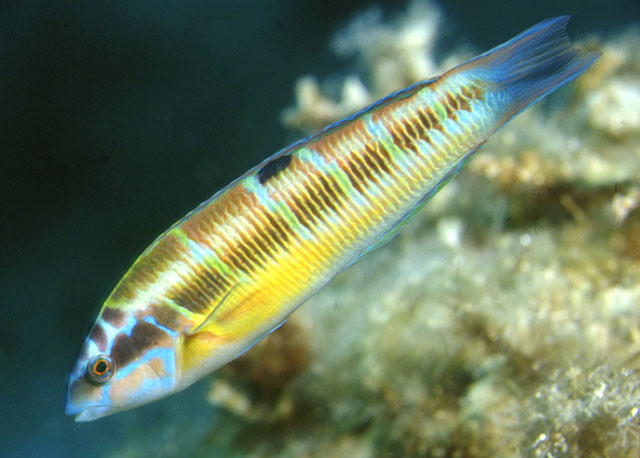
Fit a Linear Model to Reef Fish Data
-
lm()is the basic linear model function in R. - Let’s do a linear model on our fish species with temperature as a predictor
mod <- lm(
  AbundanceAdult40 ~ MeanTemp_CoralWatch,
  data = fish_dat)
R ‘formulas’
mod <- lm(
  ### <b>
  AbundanceAdult40 ~ MeanTemp_CoralWatch,
  ### </b>
data = fish_dat)- A formula is a special data structure in R
- It is specified using an expression of this form:
lhs ~ rhs, wherelhsstands for Left Hand Side, andrhsstands for Right Hand Side. - Formulas compactly express a relationship between variables:
lhscontains ‘response’ variables that we wish to model as a function of the variables on therhs: the ‘predictor’ variable - Both
lhsandrhscan contain multiple variables and function calls (we will see examples of that later on) - Though a formula can be missing
lhs, they must always have a~and arhs(~ rhsis a valid formula)
summary(mod)##
## Call:
## lm(formula = AbundanceAdult40 ~ MeanTemp_CoralWatch, data = fish_dat)
##
## Residuals:
## Min 1Q Median 3Q Max
## -42.81 -14.23 -9.13 -2.93 898.16
##
## Coefficients:
## Estimate Std. Error t value Pr(>|t|)
## (Intercept) -47.326 22.506 -2.103 0.03614 *
## MeanTemp_CoralWatch 3.274 1.147 2.853 0.00457 **
## ---
## Signif. codes: 0 '***' 0.001 '**' 0.01 '*' 0.05 '.' 0.1 ' ' 1
##
## Residual standard error: 54.3 on 383 degrees of freedom
## Multiple R-squared: 0.02081, Adjusted R-squared: 0.01825
## F-statistic: 8.139 on 1 and 383 DF, p-value: 0.004567Fit a Linear Model to Reef Fish Data
ggplot(fish_dat, aes(x = MeanTemp_CoralWatch, y = AbundanceAdult40)) +
  geom_smooth(method = lm, se = FALSE, color = "red") + geom_point() + theme_minimal()
## `geom_smooth()` using formula 'y ~ x'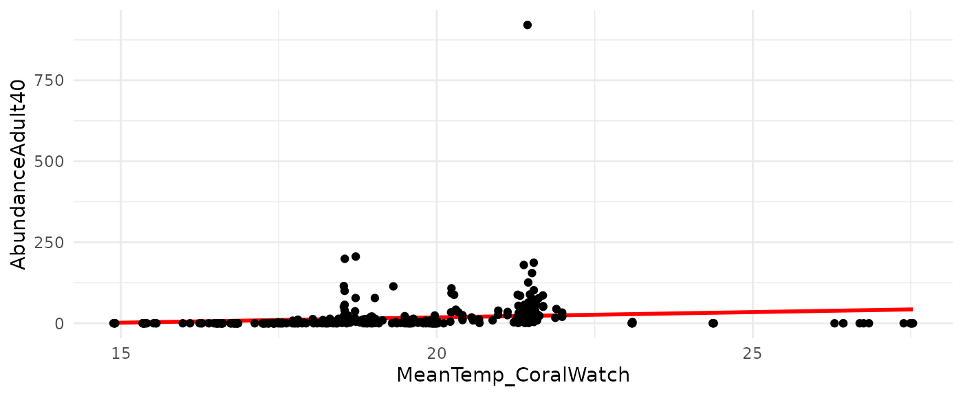
It is much easier to tell if the model is useful at all by visualizing.
Fit a Linear Model to Reef Fish Data
- This model is not a good fit, and there might be some other problems
- Models have assumptions
- Does our data fit the assumptions?
- I won’t go through all linear model assumption, but one is that the distribution of the data is not too extreme (skewed, or with long tails)
Fit a Linear Model to Reef Fish Data
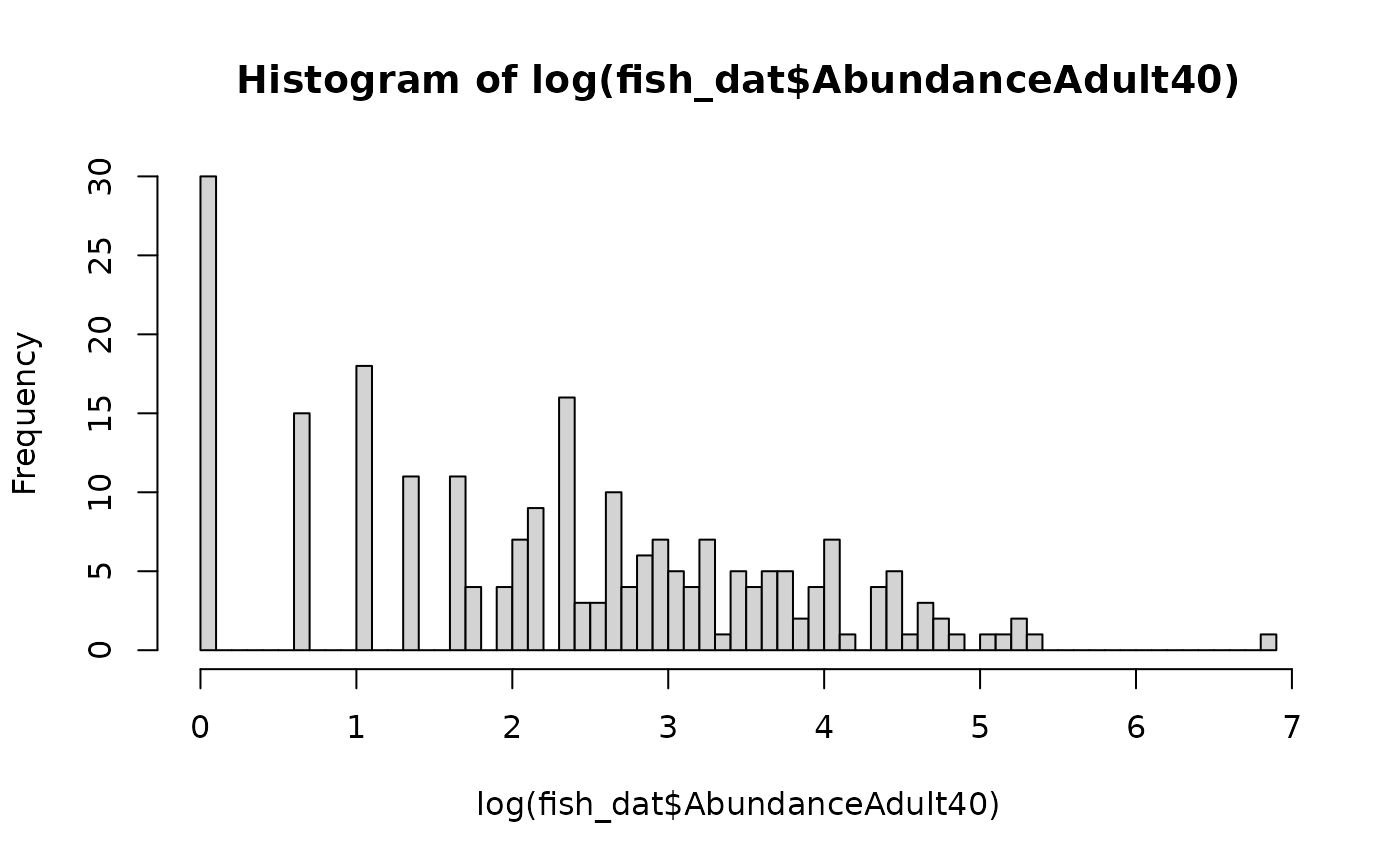
Distribution of Abundance:
hist(fish_dat$AbundanceAdult40, breaks = 100)
Fit a Linear Model to Reef Fish Data
- One way to ‘fix’ the data is to transform it, for example:
However the main problem seems to stem from the fact that a line is not a good description on the response. Therefore, most SDM methods that are actually used allow for non-linear relationships. In this case (and many cases), some kind of hump shaped function might make sense.
p <- ggplot(fish_dat, aes(x = MeanTemp_CoralWatch, y = AbundanceAdult40)) +
  geom_smooth(se = FALSE, color = "red") + geom_point() + theme_minimal()
suppressMessages(print(p))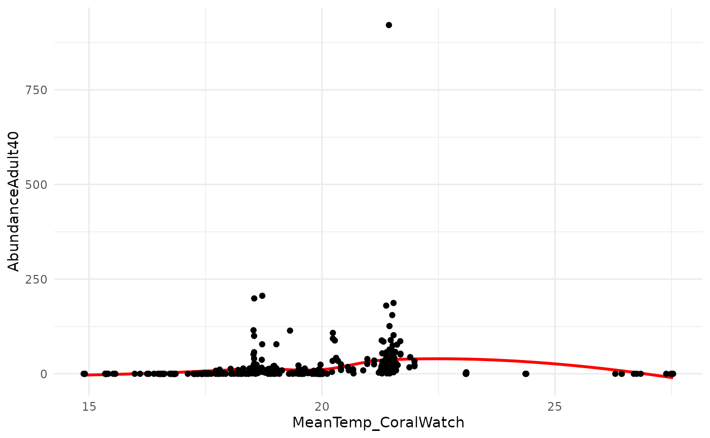
tidymodels
-
tidymodelsis an R package for statistical and machine learning models - It shares the philosophy of programming and data analysis with
tidyverse - It has functions that mirror the step of Data Science that I presented earlier
- Like
tidyverseit is a meta-package, bundling several other packages together
parsnip: a tidymodels package to fit
models
-
parsnipseparates the model ‘structure’ from the implementation - It unifies inputs and outputs, so that it is simple to switch between different modelling methods without writing new code
Fit a Linear Model with parsnip
mod_pars <- linear_reg(engine = "lm")
mod_pars
## Linear Regression Model Specification (regression)
##
## Computational engine: lmFit a Linear Model with parsnip
- A model is fit using the
fit()function -
parsnipis designed work with pipe operators (%>%or|>)
mod_pars <- linear_reg(engine = "lm") %>%
  fit(AbundanceAdult40 ~ MeanTemp_CoralWatch,
      data = fish_dat)
mod_pars
## parsnip model object
##
##
## Call:
## stats::lm(formula = AbundanceAdult40 ~ MeanTemp_CoralWatch, data = data)
##
## Coefficients:
## (Intercept) MeanTemp_CoralWatch
## -47.326 3.274Fit a Linear Model with parsnip
- Parameters are extracted with the
tidy()function.
mod_summ <- tidy(mod_pars)
mod_summ
## # A tibble: 2 × 5
## term estimate std.error statistic p.value
## <chr> <dbl> <dbl> <dbl> <dbl>
## 1 (Intercept) -47.3 22.5 -2.10 0.0361
## 2 MeanTemp_CoralWatch 3.27 1.15 2.85 0.00457Fit a Linear Model with parsnip
- Visualize the fit by prediction
preds <- predict(mod_pars, new_data = fish_dat)
preds
## # A tibble: 385 × 1
## .pred
## <dbl>
## 1 9.92
## 2 13.4
## 3 13.4
## 4 14.6
## 5 13.4
## 6 13.4
## 7 14.4
## 8 13.3
## 9 14.4
## 10 14.9
## # … with 375 more rows
p <- ggplot(pred_dat, aes(x = MeanTemp_CoralWatch, y = .pred)) +
  geom_line() + geom_point(aes(y = AbundanceAdult40)) +
  theme_minimal()
suppressMessages(print(p))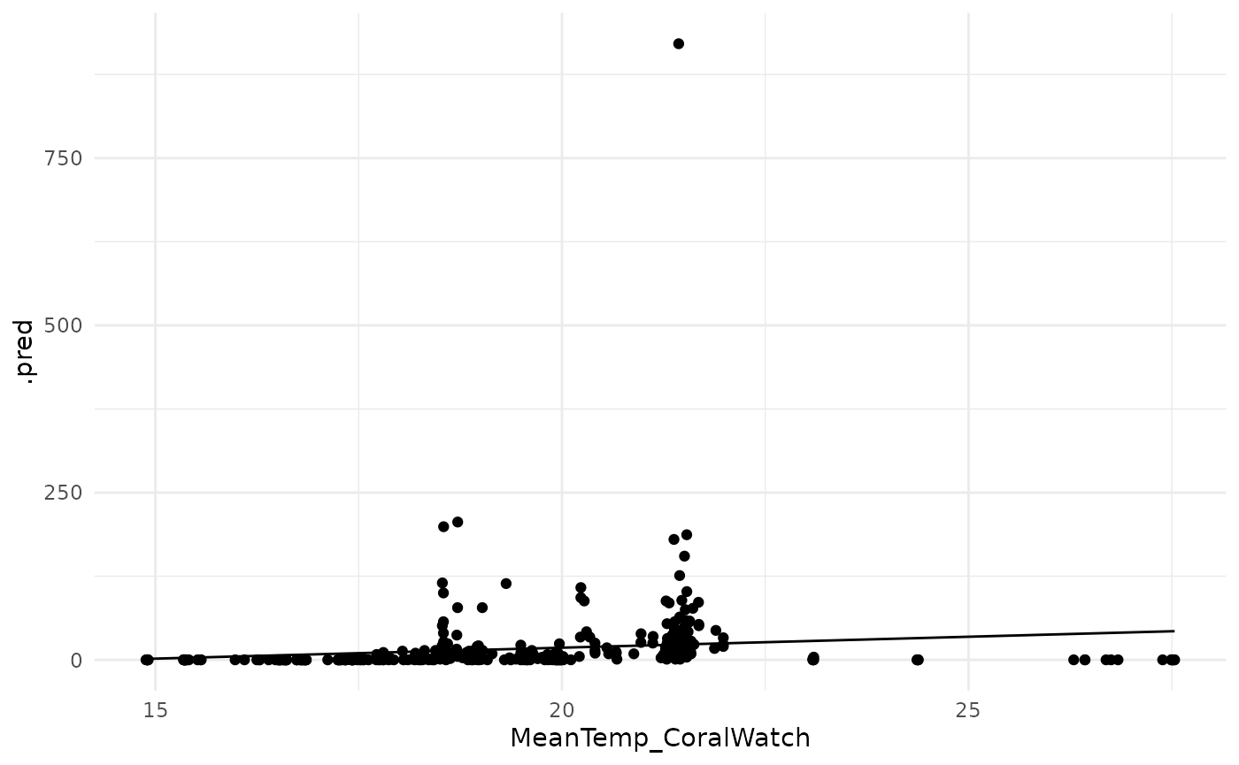
p <- ggplot(pred_dat, aes(x = MeanTemp_CoralWatch, y = .pred)) +
  geom_line() + geom_point(aes(y = AbundanceAdult40)) +
  scale_y_continuous(trans = "log1p") + theme_minimal()
suppressMessages(print(p))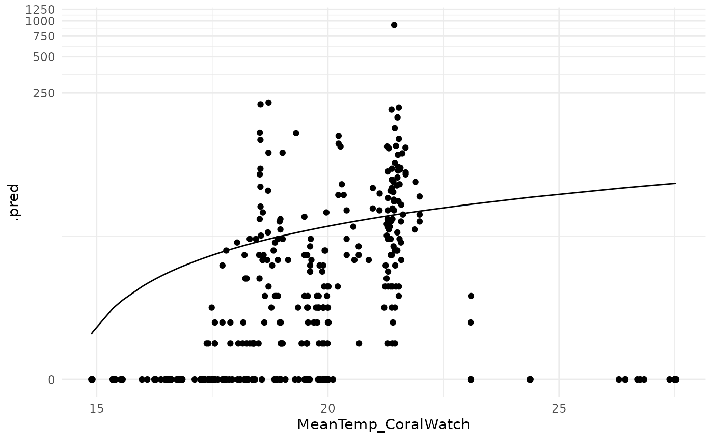
The power of parsnip
- Now that the model is specified in
parsnip, it is easy to change our model to one that can model nonlinear relationships easily. Let’s try doing a gradient boosted decision tree (you don’t need to know what that is for now).
mod_pars2 <- boost_tree(mode = "regression") %>%
  fit(AbundanceAdult40 ~ MeanTemp_CoralWatch,
      data = fish_dat)
mod_pars2
## parsnip model object
##
## ##### xgb.Booster
## raw: 47.7 Kb
## call:
## xgboost::xgb.train(params = list(eta = 0.3, max_depth = 6, gamma = 0,
## colsample_bytree = 1, colsample_bynode = 1, min_child_weight = 1,
## subsample = 1), data = x$data, nrounds = 15, watchlist = x$watchlist,
## verbose = 0, nthread = 1, objective = "reg:squarederror")
## params (as set within xgb.train):
## eta = "0.3", max_depth = "6", gamma = "0", colsample_bytree = "1", colsample_bynode = "1", min_child_weight = "1", subsample = "1", nthread = "1", objective = "reg:squarederror", validate_parameters = "TRUE"
## xgb.attributes:
## niter
## callbacks:
## cb.evaluation.log()
## # of features: 1
## niter: 15
## nfeatures : 1
## evaluation_log:
## iter training_rmse
## 1 48.35573
## 2 41.50986
## ---
## 14 13.99279
## 15 13.68966The power of parsnip
p <- ggplot(pred_dat2, aes(x = MeanTemp_CoralWatch, y = .pred)) +
  geom_line() + geom_point(aes(y = AbundanceAdult40)) +
  scale_y_continuous(trans = "log1p") + theme_minimal()
suppressMessages(print(p))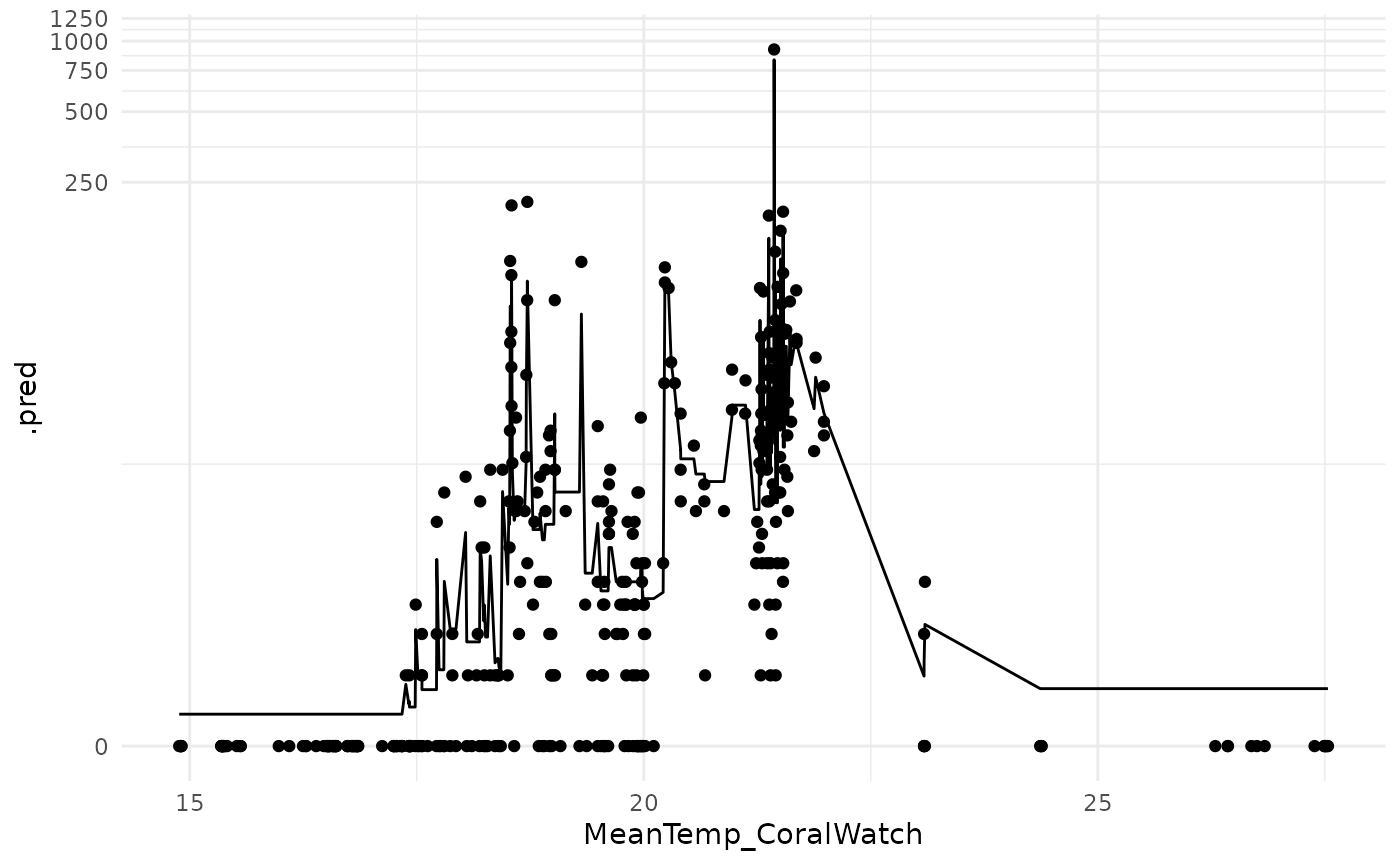
Overfitting
An important concept in Data Science and Machine Learning is the idea of overfitting. The above model appears to ‘overfit’ the data – its predictions jump around wildly to try and fit each individual data point. But this in not likely to generalize well if applied to a new dataset. We reduce overfitting by tuning the ‘hyper-parameters’ of the algorithm to make it produce ‘smoother’ predictions. Smoothed prediction are more likely to generalize better to new datasets. This is accomplished using a method called cross-validation, which we will cover in depth in Week 7.
Forests of the Future or Forests of the Past?
Introducing the Pine Rocklands of South Florida
- Unique to South Florida
- High species diversity
- Open canopy forests dominated by Slash Pine
- Fire dependent ecosystem
- One of the most critically endanger ecosystems in the world
- Why?
- Pine Rocklands central range is in the middle of Miami!
- The only large patch remaining is in Everglades National Park
knitr::include_graphics("images/pine_rockland_map.jpg")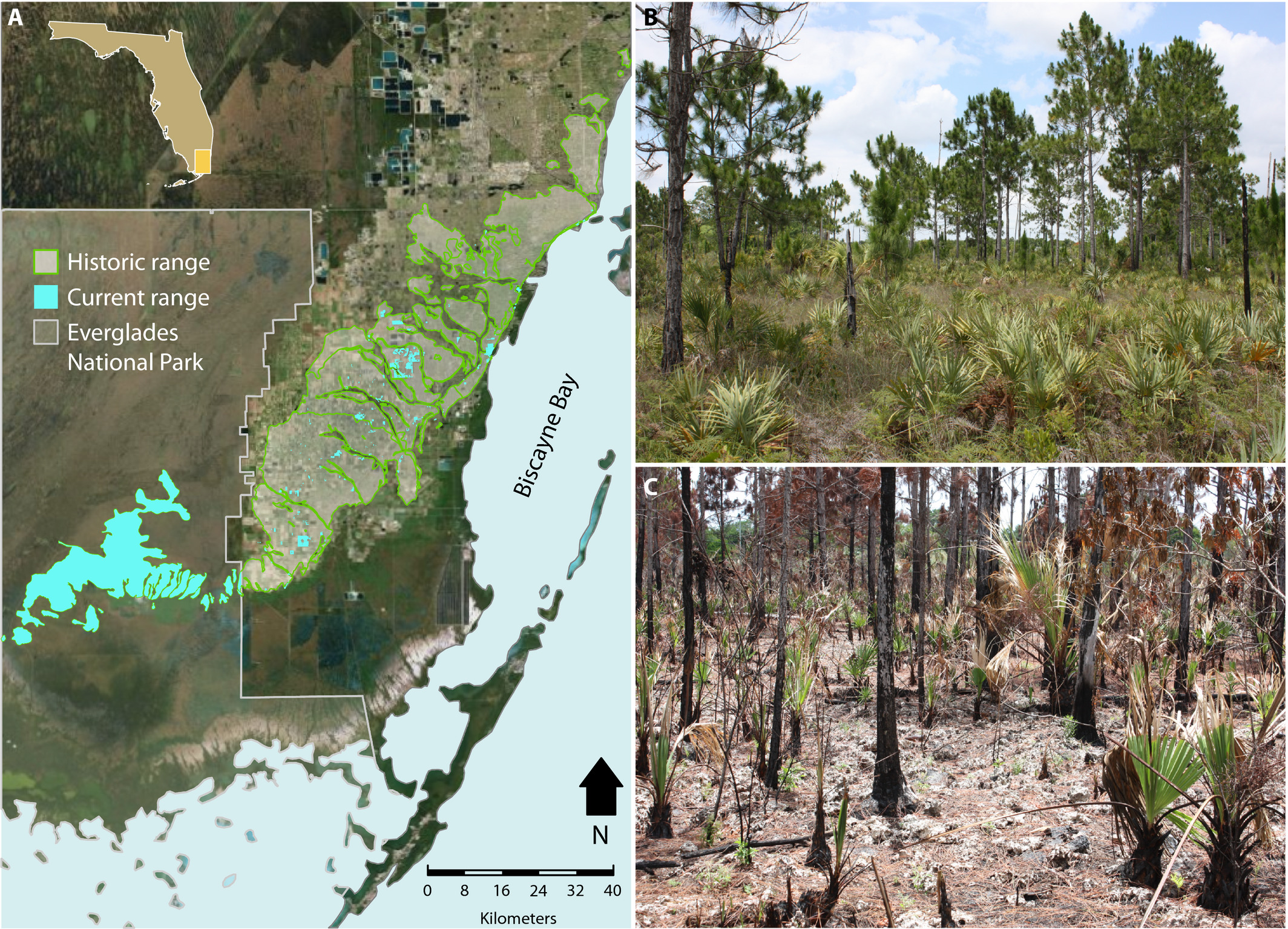
Image citation:
Trotta, Lauren B., et al. “Community phylogeny of the globally critically imperiled pine rockland ecosystem.” American journal of botany 105.10 (2018): 1735-1747.
FIU’s Pine Rockland
- The FIU Preserve on campus has one of the few remaining patches of Pine Rockland in Miami-Dade
- In 2016 FIU conducted a prescribed burn to help restore this ecosystem of local importance
Project Proposal
- I propose we do one big group project on the Pine Rocklands in weeks 11-16
- We will start here in lecture – I will use data on plants in the Pine Rockland for my examples in the next few weeks.
- For the final project, each of you can choose a species from the Pine Rocklands (or a few species) to run a SDM on and use it to make predictions. What is the past and future of Pine Rockland species?
- You will all follow the same steps of good Data Science
- You can work in groups or on your own, it is your decision
- At the end of the semester we will combine everyone’s SDMs into a prediction for the whole Pine Rockland community (or at least 18-30 species worth)
We will start by extracting data from this:
knitr::include_graphics("images/floristic.png")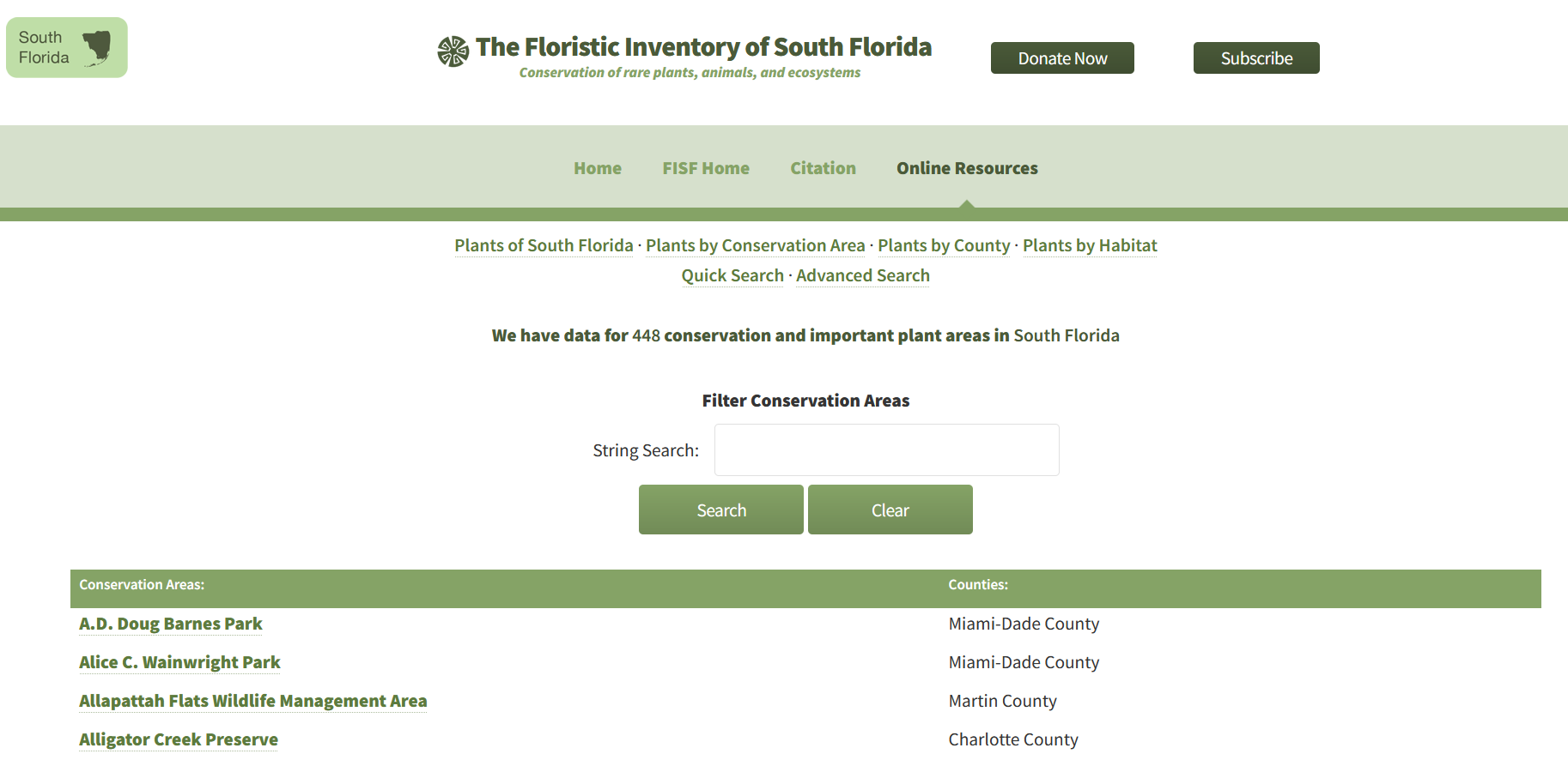
- I will start using that data for example in class next week.
- Next class we will be working on the Week 5 Assignment (you can start today).
- Next week we will cover:
- How to go from abundance data to presence / absence (e.g. occurrences)
- How to include data preprocessing and model fitting in one workflow
using
tidymodels - A little bit of ecological niche theory to understand what SDMs represent and why they are important