Forests of the Future Week 6 Lecture

Forests of the Future Week 6

Species Distribution Modelling 2

Last week we learned how to use tidymodels to fit a model to data
We modelled the abundance of fish species at different reefs based on their mean temperatures
Today we will talk about modelling occurrence data, where we have data on the presence or absence of species at particular sites
We will also learn how to preprocess data using tidymodels, with the recipes package

Ecological Niche Theory

All species have an ecological niche
An Ecological niche is the position of a species within an ecosystem
- The conditions necessary for persistence of the species
- Its ecological role in the ecosystem
Combining both more formally:
- A niche is: the part of ecological space (defined by all combinations of biotic and abiotic environmental conditions) where the species population can persist and thus utilize resources and impact its environment

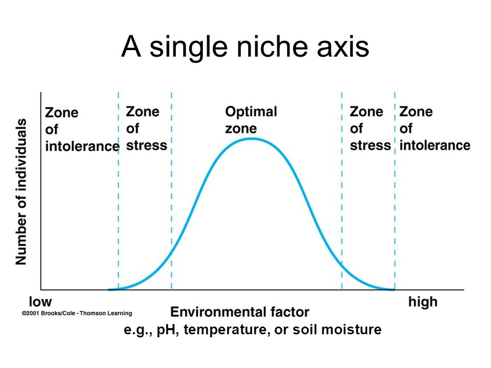
Ecological Niche Theory

Niches are often visualized or conceptualized as hump-shaped distributions along an environmental variable

Ecological Niche Theory

Compare that with the model predictions I made in last lecture:

Generalise to many dimensions

Environmental ‘hypervolume’

3D Hypervolume

Review

Data Science Steps

A Question
Collect Data
Munge / Clean Data
Transform Data for Model
Analyze Data using Model
Tune Model
Validate / Test Model
Interpret Model

This week

A Question
Collect Data
Munge / Clean Data
Transform Data for Model
Analyze Data using Model
Tune Model
Validate / Test Model
Interpret Model

Modelling fish abundance

data("RF_abund")
fish_dat <- RF_abund %>%
  filter(SpeciesName == "Thalassoma pavo") %>%
  mutate(Presence = as.factor(Presence))

What if we only had presence / absence data?

Presence / Absence Data

We are not really modelling numeric data anymore
Presence or Absence are categories
We do a classification Model, and classify into the present or absent category
Binary classification models typically output a ‘probability’, a number between 0 and 1
Observed data is compared to output using the ‘binomial’ probability distribution

Presence / Absence Data

R has a number of probability distribution built-in which we can use to explore

rbinom(100, 1, 0.5)

##   [1] 1 0 0 0 1 0 0 1 1 1 0 0 1 1 1 1 1 0 1 0 0 1 1 0 1 0 1 1 1 0 0 0 0 1 0 0 1
##  [38] 1 0 1 0 0 0 1 1 1 1 1 1 0 0 1 1 0 0 0 1 0 0 1 0 0 0 0 0 1 1 1 0 0 1 1 0 1
##  [75] 1 1 0 1 0 1 0 0 0 0 0 1 0 1 1 0 0 0 0 0 1 0 0 1 0 1

rbinom(100, 1, 0.75)

##   [1] 1 1 1 1 1 0 0 0 1 1 1 0 1 1 1 1 1 1 0 0 1 1 0 1 1 0 0 0 1 1 1 0 0 0 1 0 1
##  [38] 0 1 1 1 1 1 0 1 1 0 1 0 1 0 1 1 1 0 1 0 1 1 1 1 1 1 1 1 1 1 1 1 1 1 0 1 1
##  [75] 1 0 0 1 1 1 1 1 0 1 1 1 0 1 1 1 1 0 1 1 1 0 1 1 1 0

rbinom(100, 1, 0.25)

##   [1] 0 0 0 0 0 1 0 0 0 0 1 0 1 0 0 0 0 0 0 0 0 0 0 1 0 1 1 1 0 0 0 0 0 0 0 0 1
##  [38] 1 0 0 0 0 0 0 1 1 1 0 1 0 1 1 0 0 0 0 0 1 0 0 0 1 0 0 1 0 0 1 0 0 0 0 1 0
##  [75] 0 0 0 0 0 1 0 0 0 0 1 0 0 1 0 0 0 0 0 0 0 0 1 0 0 0

curve(dbinom(x, size = 100, 0.5), 0, 100)

`RF_abund` includes presence/absence data column

fish_dat$Presence

##   [1] 1 1 1 1 1 1 0 1 1 1 0 1 1 1 1 1 0 1 1 1 1 1 1 1 1 1 1 1 1 0 1 1 0 1 1 1 0
##  [38] 1 1 1 1 1 1 0 0 0 1 1 0 1 0 0 1 1 1 0 1 1 0 1 0 0 1 1 1 0 0 0 0 0 0 1 1 1
##  [75] 1 1 1 1 0 0 0 1 1 1 1 1 0 1 1 0 0 1 0 1 1 1 1 1 1 1 1 1 1 1 1 1 1 1 1 1 1
## [112] 1 1 1 1 1 1 1 1 1 1 1 1 1 1 1 1 1 1 1 1 1 1 1 1 1 1 1 1 1 1 1 1 1 1 1 1 1
## [149] 1 1 1 1 1 1 1 1 1 1 1 1 1 1 1 1 1 1 1 1 1 1 1 1 1 1 1 1 1 1 1 1 1 1 1 1 1
## [186] 1 1 1 1 1 1 1 1 1 1 1 1 1 1 0 0 0 0 0 1 0 0 0 0 0 0 1 1 0 1 0 0 0 0 0 0 0
## [223] 0 0 1 1 1 0 0 0 1 0 1 1 0 0 1 1 0 0 0 1 0 1 1 1 0 1 1 1 1 1 0 0 0 0 0 0 0
## [260] 0 0 0 0 0 0 0 0 0 0 0 0 1 0 0 1 0 0 0 0 0 0 0 0 0 0 0 0 0 0 0 0 1 1 0 0 1
## [297] 1 0 0 0 0 1 1 1 1 1 1 1 1 1 1 1 1 1 1 1 1 1 0 0 1 0 1 1 1 1 0 0 0 0 0 0 0
## [334] 0 0 0 0 0 0 0 0 0 0 0 0 0 0 0 0 0 0 0 0 0 0 0 0 0 0 0 0 0 0 0 0 1 1 1 0 0
## [371] 0 1 0 0 1 1 1 1 1 0 1 0 0 0 1
## Levels: 0 1

Let’s model fish occurrence

Use two variables: Mean Temperature and Depth
In order to make them more comparable we will ‘standardise’ them
We will also test our model by creating a test set

Split off a test set:

set.seed(1234)
data_split <- initial_split(fish_dat, 0.8, strata = Presence)

train_data <- training(data_split)
test_data <- testing(data_split)

train_data

## # A tibble: 308 × 25
##    SpeciesName   SiteC…¹ Abund…² Sampl…³ MeanT…⁴ MinTe…⁵ MaxTe…⁶ SDTem…⁷ ECOre…⁸
##    <chr>         <chr>     <dbl>   <dbl>   <dbl>   <dbl>   <dbl>   <dbl> <fct>  
##  1 Thalassoma p… AND2          0     164    17.6    14.1    22.8    2.85 Albora…
##  2 Thalassoma p… AND25         0     173    19.0    14.0    25.4    4.01 Albora…
##  3 Thalassoma p… AND37         0     173    19.1    14.0    26.1    4.20 Albora…
##  4 Thalassoma p… AND43         0     173    18.9    14.3    25.3    3.66 Albora…
##  5 Thalassoma p… AND50         0     164    18.2    14.2    23.5    3.02 Albora…
##  6 Thalassoma p… AND51         0     164    18.3    14.1    23.8    3.12 Albora…
##  7 Thalassoma p… AND54         0     173    18.6    14.2    24.6    3.41 Albora…
##  8 Thalassoma p… AND56         0     164    17.8    14.2    22.1    2.66 Albora…
##  9 Thalassoma p… AND60         0     164    18.4    14.9    22.2    2.53 Sahara…
## 10 Thalassoma p… AND63         0     173    18.9    14.4    26.3    3.85 Albora…
## # … with 298 more rows, 16 more variables: Presence <fct>, OLRE <fct>,
## #   MaxAbundance <dbl>, N_Obs <int>, Confidence_NObs <dbl>, T_Range_Obs <dbl>,
## #   Confidence_TRange_Obs <dbl>, N_Absences_T_Upper <int>,
## #   N_Absences_T_Lower <int>, Confidence_Occ_Tupper <dbl>,
## #   Confidence_Occ_Tlower <dbl>, T_Upper_Absences <dbl>,
## #   T_Lower_Absences <dbl>, T_Mean_Absences <dbl>, NEOLI <dbl>,
## #   Depth_Site <dbl>, and abbreviated variable names ¹SiteCode, …

test_data

## # A tibble: 77 × 25
##    SpeciesName   SiteC…¹ Abund…² Sampl…³ MeanT…⁴ MinTe…⁵ MaxTe…⁶ SDTem…⁷ ECOre…⁸
##    <chr>         <chr>     <dbl>   <dbl>   <dbl>   <dbl>   <dbl>   <dbl> <fct>  
##  1 Thalassoma p… AND1          3     217    17.5    14.1    22.6    2.75 Albora…
##  2 Thalassoma p… AND12       100     173    18.5    14.0    24.7    3.67 Albora…
##  3 Thalassoma p… AND16         0     173    18.8    14.0    25.2    3.89 Albora…
##  4 Thalassoma p… AND18        13     173    18.9    14.0    25.2    3.92 Albora…
##  5 Thalassoma p… AND19         1     173    19.0    14.0    25.5    4.08 Albora…
##  6 Thalassoma p… AND21        11     173    18.8    14.0    25.2    3.87 Albora…
##  7 Thalassoma p… AND27        14     173    19.0    14.0    25.5    4.08 Albora…
##  8 Thalassoma p… AND29        17     173    19.0    14.0    25.4    4.03 Albora…
##  9 Thalassoma p… AND3          8     164    17.7    14.1    22.9    2.90 Albora…
## 10 Thalassoma p… AND4          0     164    17.9    14.1    23.3    3.01 Albora…
## # … with 67 more rows, 16 more variables: Presence <fct>, OLRE <fct>,
## #   MaxAbundance <dbl>, N_Obs <int>, Confidence_NObs <dbl>, T_Range_Obs <dbl>,
## #   Confidence_TRange_Obs <dbl>, N_Absences_T_Upper <int>,
## #   N_Absences_T_Lower <int>, Confidence_Occ_Tupper <dbl>,
## #   Confidence_Occ_Tlower <dbl>, T_Upper_Absences <dbl>,
## #   T_Lower_Absences <dbl>, T_Mean_Absences <dbl>, NEOLI <dbl>,
## #   Depth_Site <dbl>, and abbreviated variable names ¹SiteCode, …

Transform data

Make symmetric and non-skewed (Yeo-Johnson transformation)
Flexible transformation that needs a parameter, which is usually chosen based on an optimization with the training data
Standardise (make mean zero, and standard deviation 1)
Before:

s_dat <- train_data %>%
  select(MeanTemp_CoralWatch, Depth_Site) %>%
  pivot_longer(cols = everything(), values_to = "Value", names_to = "Variable")
ggplot(s_dat, aes(Value)) +
  geom_histogram(bins = 30) +
  facet_wrap(vars(Variable), nrow = 2, scales = "free") +
  theme_minimal()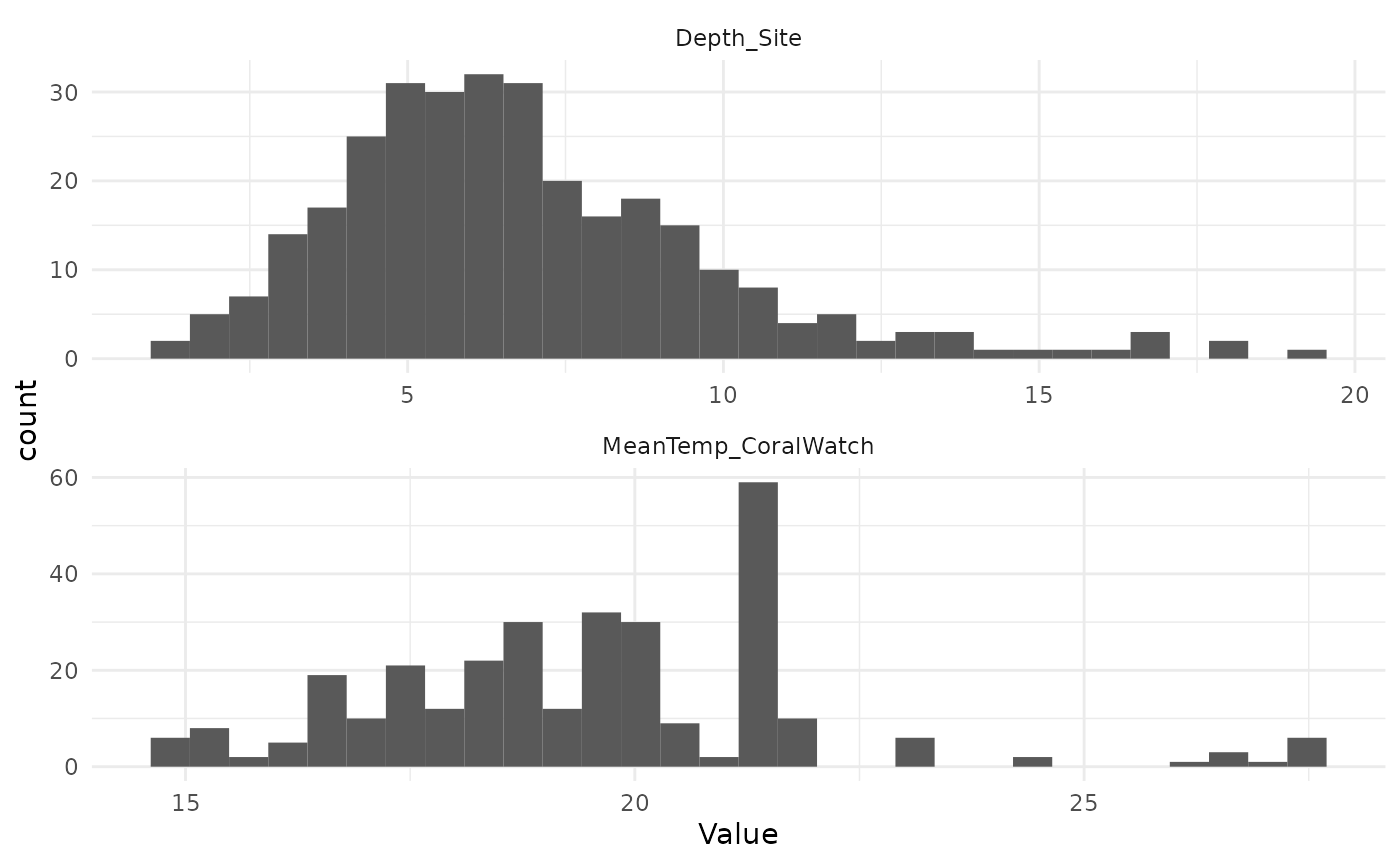

MeanTemp_yj <- car::powerTransform(train_data$MeanTemp_CoralWatch,
                                   family = "yjPower")
Depth_yj <- car::powerTransform(train_data$Depth_Site,
                                family = "yjPower")
MeanTemp_yj

## Estimated transformation parameter 
## train_data$MeanTemp_CoralWatch 
##                     -0.8426166

Depth_yj

## Estimated transformation parameter 
## train_data$Depth_Site 
##             0.1361994

train_data <- train_data %>%
  mutate(MeanTemp_tr = car::yjPower(MeanTemp_CoralWatch, MeanTemp_yj$roundlam),
         Depth_tr = car::yjPower(Depth_Site, Depth_yj$roundlam))

After:

s_dat <- train_data %>%
  select(MeanTemp_tr, Depth_tr) %>%
  pivot_longer(cols = everything(), values_to = "Value", names_to = "Variable")
ggplot(s_dat, aes(Value)) +
  geom_histogram(bins = 30) +
  facet_wrap(vars(Variable), nrow = 2, scales = "free") +
  theme_minimal()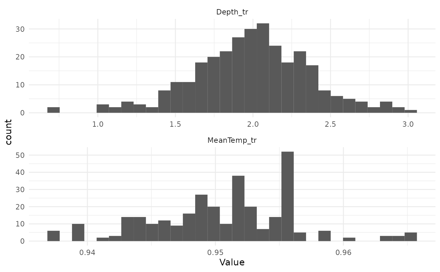

What about the test data?

When we use the model to predict the occurrence on the test set, the data must be transformed in exactly the same way as the training set
This means we need to keep our lambda parameter fit on the training data and apply the same parameter to transform the test data
The standardisation also requires parameters from the training data
Keeping track of these transformations manually is dangerous
A common mistake is to transform the test data using parameters derived from the test data, this makes the test data incomparable to the training data

Recipes helps to solve this issue

A recipe is a set of steps applied to data before modelling
Everything is kept track of by tidymodels so that the steps are applied correctly to test data after the model is fit
Let’s make a recipe

RF_recipe <- recipe(train_data,
                    Presence ~ MeanTemp_CoralWatch + Depth_Site)
RF_recipe

## Recipe
## 
## Inputs:
## 
##       role #variables
##    outcome          1
##  predictor          2

Add Steps to the `recipe`

RF_recipe <- recipe(train_data,
                    Presence ~ MeanTemp_CoralWatch + Depth_Site) %>%
  step_YeoJohnson(MeanTemp_CoralWatch, Depth_Site) %>%
  step_normalize(MeanTemp_CoralWatch, Depth_Site)
RF_recipe

## Recipe
## 
## Inputs:
## 
##       role #variables
##    outcome          1
##  predictor          2
## 
## Operations:
## 
## Yeo-Johnson transformation on MeanTemp_CoralWatch, Depth_Site
## Centering and scaling for MeanTemp_CoralWatch, Depth_Site

Prep the `recipe`

Prepping a recipe estimates any required parameters

RF_recipe <- prep(RF_recipe)
RF_recipe

## Recipe
## 
## Inputs:
## 
##       role #variables
##    outcome          1
##  predictor          2
## 
## Training data contained 308 data points and no missing data.
## 
## Operations:
## 
## Yeo-Johnson transformation on MeanTemp_CoralWatch, Depth_Site [trained]
## Centering and scaling for MeanTemp_CoralWatch, Depth_Site [trained]

Bake the `recipe`

Baking applies the steps to a dataset

train_data_tr <- bake(RF_recipe, train_data)
train_data_tr

## # A tibble: 308 × 3
##    MeanTemp_CoralWatch Depth_Site Presence
##                  <dbl>      <dbl> <fct>   
##  1             -0.761     -1.37   0       
##  2             -0.125     -2.22   0       
##  3             -0.0707     0.555  0       
##  4             -0.150     -1.34   0       
##  5             -0.480     -1.73   0       
##  6             -0.448     -0.645  0       
##  7             -0.300     -0.946  0       
##  8             -0.672      0.144  0       
##  9             -0.369     -0.196  0       
## 10             -0.159     -0.0482 0       
## # … with 298 more rows

The data now looks like:

s_dat <- train_data_tr %>% select(MeanTemp_CoralWatch, Depth_Site) %>% pivot_longer(cols = everything(), values_to = "Value", names_to = "Variable")
ggplot(s_dat, aes(Value)) + geom_histogram(bins = 30) + facet_wrap(vars(Variable), nrow = 2, scales = "free") + theme_minimal()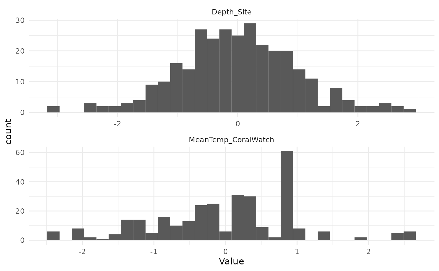

Bake the test data

We can now easily apply the exact same data manipulation to the test data

test_data_tr <- bake(RF_recipe, test_data)
test_data_tr

## # A tibble: 77 × 3
##    MeanTemp_CoralWatch Depth_Site Presence
##                  <dbl>      <dbl> <fct>   
##  1             -0.828    -2.00    1       
##  2             -0.315     0.00543 1       
##  3             -0.177    -0.412   0       
##  4             -0.171     0.495   1       
##  5             -0.0972   -2.00    1       
##  6             -0.185    -0.667   1       
##  7             -0.0980   -1.93    1       
##  8             -0.119     0.178   1       
##  9             -0.710    -3.14    1       
## 10             -0.637    -2.64    0       
## # … with 67 more rows

Combine a `recipe` and a `model`

RF_mod <-
  boost_tree() %>%
  set_engine('xgboost') %>%
  set_mode('classification')

RF_mod

## Boosted Tree Model Specification (classification)
## 
## Computational engine: xgboost

A `workflow` is a `recipe` and a `model`

RF_wf <- workflow() %>%
  add_recipe(RF_recipe) %>%
  add_model(RF_mod)

RF_wf

## ══ Workflow ════════════════════════════════════════════════════════════════════
## Preprocessor: Recipe
## Model: boost_tree()
## 
## ── Preprocessor ────────────────────────────────────────────────────────────────
## 2 Recipe Steps
## 
## • step_YeoJohnson()
## • step_normalize()
## 
## ── Model ───────────────────────────────────────────────────────────────────────
## Boosted Tree Model Specification (classification)
## 
## Computational engine: xgboost

Use `fit` to run a workflow

RF_fit <- RF_wf %>%
  fit(train_data)

RF_fit

## ══ Workflow [trained] ══════════════════════════════════════════════════════════
## Preprocessor: Recipe
## Model: boost_tree()
## 
## ── Preprocessor ────────────────────────────────────────────────────────────────
## 2 Recipe Steps
## 
## • step_YeoJohnson()
## • step_normalize()
## 
## ── Model ───────────────────────────────────────────────────────────────────────
## ##### xgb.Booster
## raw: 25.1 Kb 
## call:
##   xgboost::xgb.train(params = list(eta = 0.3, max_depth = 6, gamma = 0, 
##     colsample_bytree = 1, colsample_bynode = 1, min_child_weight = 1, 
##     subsample = 1), data = x$data, nrounds = 15, watchlist = x$watchlist, 
##     verbose = 0, nthread = 1, objective = "binary:logistic")
## params (as set within xgb.train):
##   eta = "0.3", max_depth = "6", gamma = "0", colsample_bytree = "1", colsample_bynode = "1", min_child_weight = "1", subsample = "1", nthread = "1", objective = "binary:logistic", validate_parameters = "TRUE"
## xgb.attributes:
##   niter
## callbacks:
##   cb.evaluation.log()
## # of features: 2 
## niter: 15
## nfeatures : 2 
## evaluation_log:
##     iter training_logloss
##        1        0.5244973
##        2        0.4279284
## ---                      
##       14        0.1878803
##       15        0.1829834

Make predictions

Predict the test data
The workflow knows to apply the recipe to the test data first

predict(RF_fit, test_data)

## # A tibble: 77 × 1
##    .pred_class
##    <fct>      
##  1 0          
##  2 1          
##  3 1          
##  4 1          
##  5 1          
##  6 1          
##  7 1          
##  8 1          
##  9 0          
## 10 0          
## # … with 67 more rows

predict(RF_fit, test_data, type = "prob")

## # A tibble: 77 × 2
##    .pred_0 .pred_1
##      <dbl>   <dbl>
##  1  0.916   0.0842
##  2  0.110   0.890 
##  3  0.118   0.882 
##  4  0.0654  0.935 
##  5  0.224   0.776 
##  6  0.0807  0.919 
##  7  0.224   0.776 
##  8  0.136   0.864 
##  9  0.879   0.121 
## 10  0.767   0.233 
## # … with 67 more rows

Augment data with predictions

RF_test_preds <- augment(RF_fit, test_data)

At last we test the fit based on test data

RF_test_preds %>% 
  roc_curve(.pred_0, truth = Presence) %>% 
  autoplot()

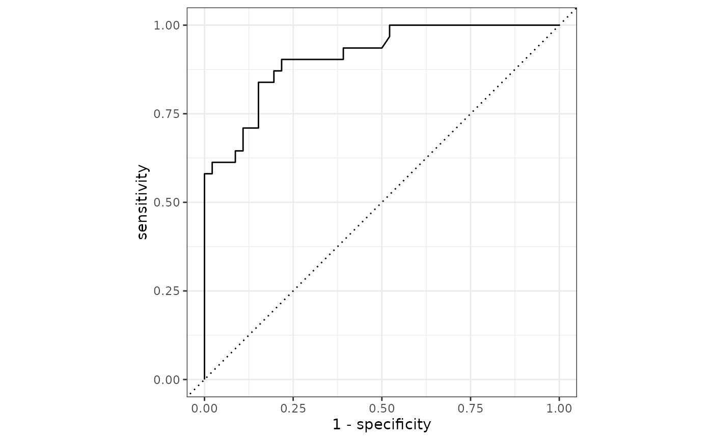
RF_test_preds %>% 
  roc_auc(.pred_0, truth = Presence)

## # A tibble: 1 × 3
##   .metric .estimator .estimate
##   <chr>   <chr>          <dbl>
## 1 roc_auc binary         0.911

Plot predictions and original data

pred_dat <- cross_df(list(MeanTemp_CoralWatch = seq(min(fish_dat$MeanTemp_CoralWatch),
                                                    max(fish_dat$MeanTemp_CoralWatch),
                                                    length.out = 100),
                            Depth_Site = seq(min(fish_dat$Depth_Site),
                                             max(fish_dat$Depth_Site),
                                             length.out = 100)))

newdat <- augment(RF_fit, pred_dat)

ggplot(newdat, aes(MeanTemp_CoralWatch, Depth_Site)) +
  geom_contour_filled(aes(z = .pred_1)) +
  geom_point(aes(size = Presence), data = fish_dat, alpha = 0.6) +
  theme_minimal()

## Warning: Using size for a discrete variable is not advised.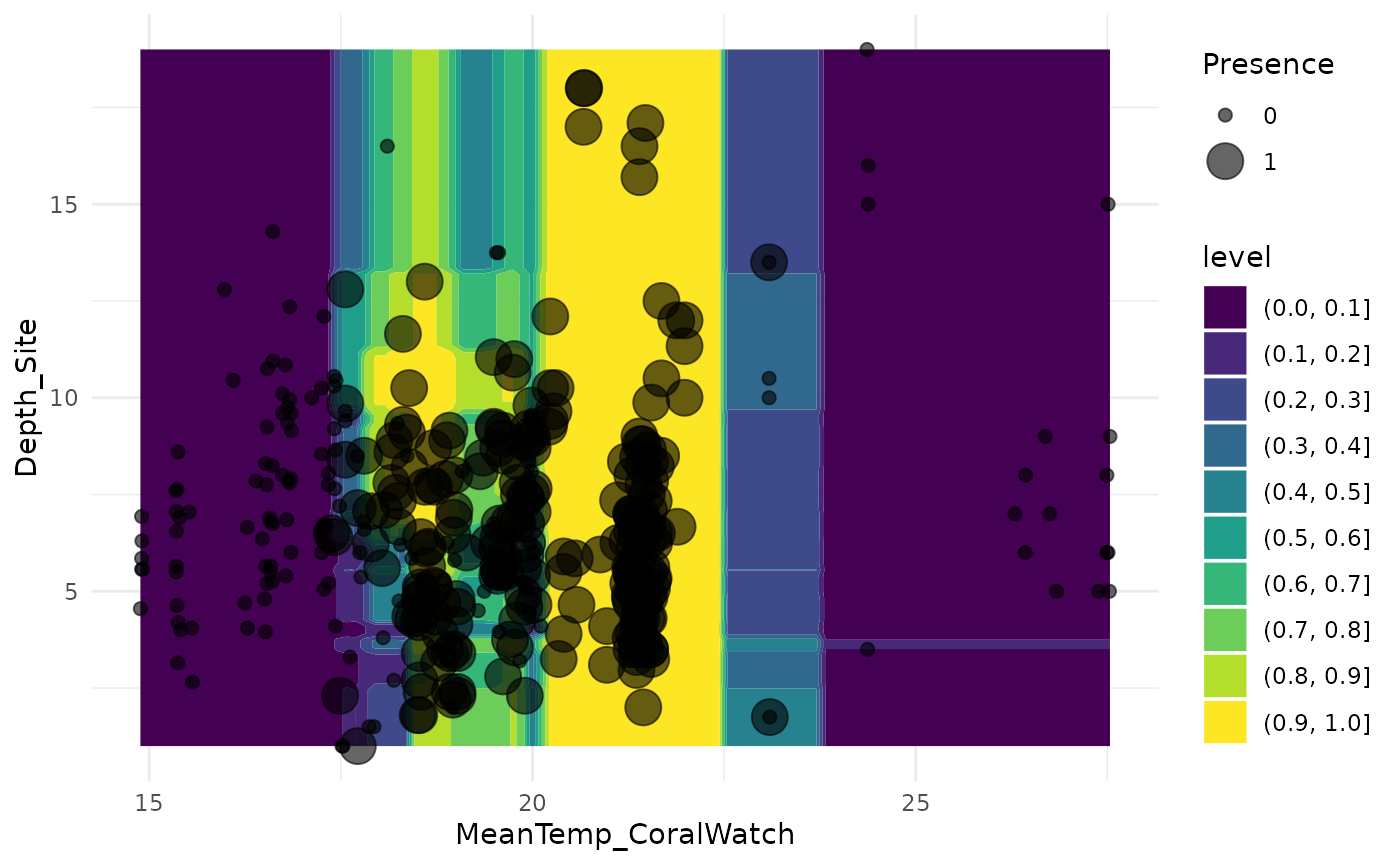

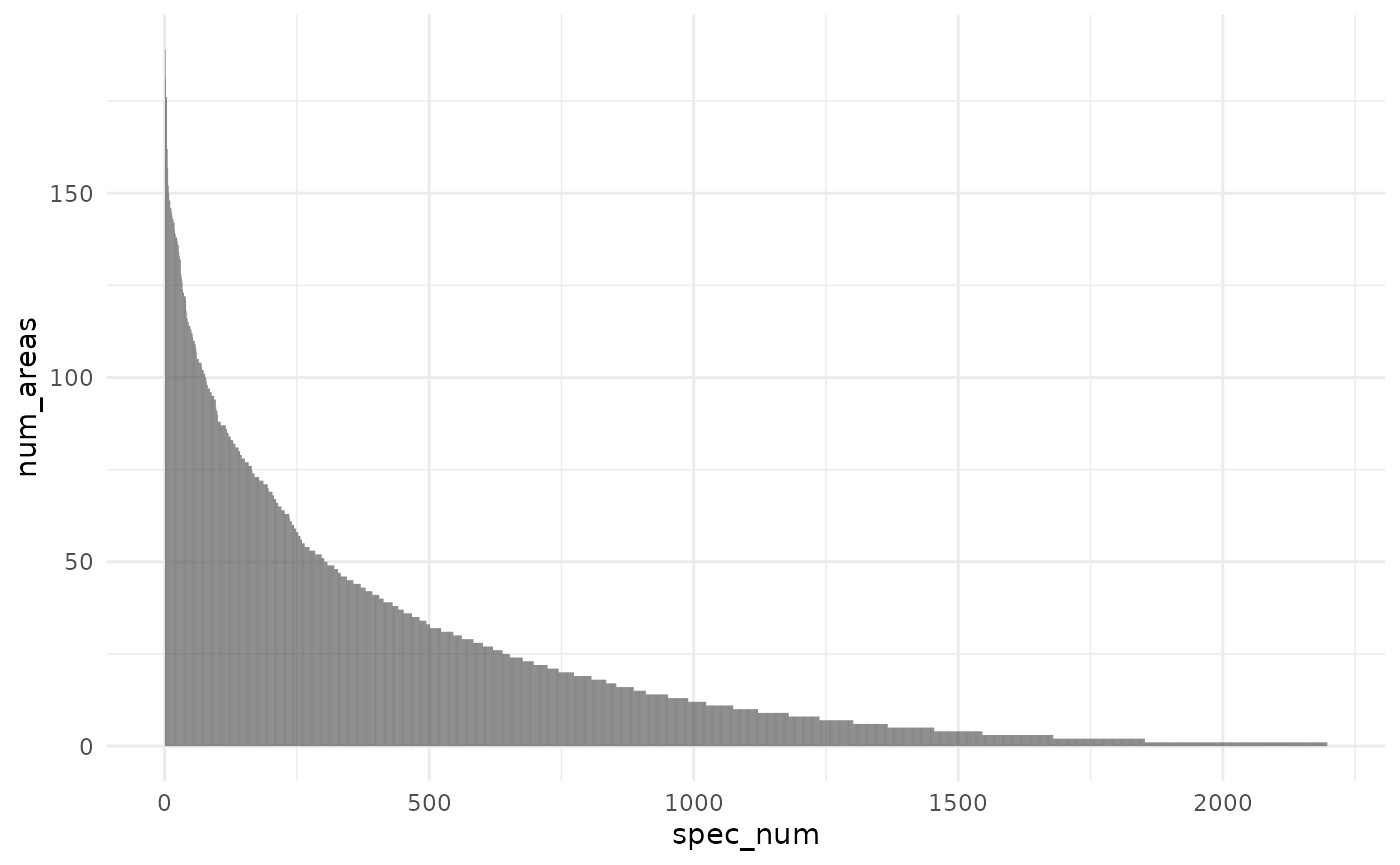
Pine Rocklands Plant Species

data("IRC")
IRC

## # A tibble: 476,255 × 7
##    ScientificName         area_name            Occur…¹ Intro…² size   long   lat
##    <chr>                  <chr>                <chr>   <chr>   <chr> <dbl> <dbl>
##  1 Abelmoschus esculentus A.D. Doug Barnes Pa… Absent  Not in… 60.4… -80.3  25.7
##  2 Abelmoschus esculentus Alice C. Wainwright… Absent  Not in… 21.5… -80.2  25.7
##  3 Abelmoschus esculentus Allapattah Flats Wi… Absent  Not in… 2094… -80.5  27.2
##  4 Abelmoschus esculentus Amberjack Slough     Absent  Not in… 182 … -82.3  26.9
##  5 Abelmoschus esculentus Arch Creek Park      Absent  Not in… 10.3… -80.2  25.9
##  6 Abelmoschus esculentus Arthur R. Marshall … Absent  Not in… 1484… -80.2  26.5
##  7 Abelmoschus esculentus Bahia Honda State P… Absent  Not in… 491.… -81.3  24.7
##  8 Abelmoschus esculentus Bartlett Estate      Absent  Not in… 35 a… -80.1  26.1
##  9 Abelmoschus esculentus Beachwalk Pasley Pa… Absent  Not in… 17 a… -80.2  27.2
## 10 Abelmoschus esculentus Big and Little Geor… Absent  Not in… 18.2… -80.4  25.6
## # … with 476,245 more rows, and abbreviated variable names ¹Occurrence,
## #   ²Introduced

Summary

n_distinct(IRC$area_name)

## [1] 205

n_distinct(IRC$ScientificName)

## [1] 2323

Species Summary

IRC_summ <- IRC %>%
  filter(Occurrence == "Present") %>%
  group_by(ScientificName) %>%
  summarise(num_areas = n_distinct(area_name)) %>%
  arrange(desc(num_areas)) %>%
  mutate(spec_num = 1:n())

ggplot(IRC_summ, aes(spec_num, num_areas)) +
  geom_col() +
  theme_minimal()

Forests of the Future Week 6

Species Distribution Modelling 2

Ecological Niche Theory

Ecological Niche Theory

Ecological Niche Theory

Generalise to many dimensions

Review

Data Science Steps

This week

Presence / Absence Data

Presence / Absence Data

RF_abund includes presence/absence data column

Let’s model fish occurrence

Transform data

What about the test data?

Recipes helps to solve this issue

Add Steps to the recipe

Prep the recipe

Bake the recipe

Bake the test data

Combine a recipe and a model

A workflow is a recipe and a model

Use fit to run a workflow

Make predictions

Augment data with predictions

At last we test the fit based on test data

Plot predictions and original data

Pine Rocklands Plant Species

Summary

Species Summary

`RF_abund` includes presence/absence data column

Add Steps to the `recipe`

Prep the `recipe`

Bake the `recipe`

Combine a `recipe` and a `model`

A `workflow` is a `recipe` and a `model`

Use `fit` to run a workflow