simple_example_using_migration_and_fst
Source:vignettes/articles/simple_example_using_migration_and_fst.Rmd
simple_example_using_migration_and_fst.Rmd
library(slimr)
#> Welcome to the slimr package for forward population genetics simulation in SLiM. For more information on SLiM please visit https://messerlab.org/slim/ .
#>
#> Attaching package: 'slimr'
#> The following object is masked from 'package:methods':
#>
#>     initialize
#> The following object is masked from 'package:base':
#>
#>     interaction
library(adegenet)
#> Loading required package: ade4
#>
#>    /// adegenet 2.1.10 is loaded ////////////
#>
#>    > overview: '?adegenet'
#>    > tutorials/doc/questions: 'adegenetWeb()'
#>    > bug reports/feature requests: adegenetIssues()
library(dartR)
#> Loading required package: ggplot2
#> Loading required package: dplyr
#>
#> Attaching package: 'dplyr'
#> The following object is masked from 'package:slimr':
#>
#>     first
#> The following objects are masked from 'package:stats':
#>
#>     filter, lag
#> The following objects are masked from 'package:base':
#>
#>     intersect, setdiff, setequal, union
#> Loading required package: dartR.data
#> Registered S3 method overwritten by 'pegas':
#>   method      from
#>   print.amova ade4
#> Registered S3 method overwritten by 'GGally':
#>   method from
#>   +.gg   ggplot2
#> Registered S3 method overwritten by 'genetics':
#>   method      from
#> [.haplotype pegasinitialize() {
initializeMutationRate(1e-7);
initializeMutationType("m1", 0.5, "f", 0.0);
initializeGenomicElementType("g1", m1, 1.0);
initializeGenomicElement(g1, 0, 99999);
initializeRecombinationRate(1e-8);
}
1 {
for (i in 1:3)
sim.addSubpop(i, 1000);
subpops = sim.subpopulations;
lines = readFile("~/Desktop/migration.csv");
lines = lines[substr(lines, 0, 1) != "//"];
for (line in lines)
{
fields = strsplit(line, ",");
i = asInteger(fields[0]);
j = asInteger(fields[1]);
m = asFloat(fields[2]);
if (i != j)
{
p_i = subpops[subpops.id == i];
p_j = subpops[subpops.id == j];
p_j.setMigrationRates(p_i, m);
}
}
}
10000 late() { sim.outputFull(); }
slim_script(
  slim_block(initialize(), {
    initializeMutationRate(1e-7);
    initializeMutationType("m1", 0.5, "f", 0.0);
    initializeGenomicElementType("g1", m1, 1.0);
    initializeGenomicElement(g1, 0, 99999);
    initializeRecombinationRate(1e-8);
  }),
  slim_block(1, {
    for (i in 1:3) {
      sim.addSubpop(i, 1000);
    }
    subpops = sim.subpopulations;
    lines = readFile("~/Desktop/migration.csv");
    lines = lines[substr(lines, 0, 1) != "//"];
    for (line in lines) {
      fields = strsplit(line, ",");
      i = asInteger(fields[0]);
      j = asInteger(fields[1]);
      m = asFloat(fields[2]);
      if (i != j) {
        p_i = subpops[subpops.id == i];
        p_j = subpops[subpops.id == j];
        p_j.setMigrationRates(p_i, m);
      }
    }
  }),
  slim_block(10000, late(), {
    sim.outputFull();
  })
) -> script_1

script_1
#> <slimr_script[3]>
#> block_init:initialize() {
#> initializeMutationRate(1e-07);
#> initializeMutationType("m1", 0.5, "f", 0);
#> initializeGenomicElementType("g1", m1, 1);
#> initializeGenomicElement(g1, 0, 99999);
#> initializeRecombinationRate(1e-08);
#> }
#>
#> block_2:1 early() {
#> for (i in 1:3) {
#> sim.addSubpop(i, 1000);
#> }
#> subpops = sim.subpopulations;
#> lines = readFile("~/Desktop/migration.csv");
#> lines = lines[substr(lines, 0, 1) != "//"];
#> for (line in lines) {
#> fields = strsplit(line, ",");
#> i = asInteger(fields[0]);
#> j = asInteger(fields[1]);
#> m = asFloat(fields[2]);
#> if (i != j) {
#> p_i = subpops[subpops.id == i];
#> p_j = subpops[subpops.id == j];
#> p_j.setMigrationRates(p_i, m);
#> }
#> }
#> }
#>
#> block_3:10000 late() {
#> sim.outputFull();
#> }
disp_mat <- matrix(c(1, 1, 0.78,
                     1, 2, 0.10,
                     1, 3, 0.12,
                     2, 1, 0.01,
                     2, 2, 0.96,
                     2, 3, 0.03,
                     3, 1, 0.33,
                     3, 2, 0.17,
                     3, 3, 0.5),
                   ncol = 3, byrow = TRUE)

slim_script(
  slim_block(initialize(), {
    setSeed(123456);
    initializeMutationRate(2e-6);
    initializeMutationType("m1", 0.5, "f", 0.0);
    initializeGenomicElementType("g1", m1, 1.0);
    initializeGenomicElement(g1, 0, 99999);
    initializeRecombinationRate(1e-8);
  }),
  slim_block(1, {
    for (i in 1:3) {
      sim.addSubpop(i, 100);
    }
    subpops = sim.subpopulations;

    disp_mat = slimr_inline(disp_mat)

    for (line in seqLen(nrow(disp_mat))) {
      i = asInteger(disp_mat[line, 0]);
      j = asInteger(disp_mat[line, 1]);
      m = asFloat(disp_mat[line, 2]);
      if (i != j) {
        p_i = subpops[subpops.id == i];
        p_j = subpops[subpops.id == j];
        p_j.setMigrationRates(p_i, m);
      }
    }
  }),
  slim_block(100000, late(), {
    slimr_output(sim.outputFull(), "final_output");
  })
) -> script_2

script_2
#> <slimr_script[3]>
#> block_init:initialize() {
#> setSeed(123456);
#> initializeMutationRate(2e-06);
#> initializeMutationType("m1", 0.5, "f", 0);
#> initializeGenomicElementType("g1", m1, 1);
#> initializeGenomicElement(g1, 0, 99999);
#> initializeRecombinationRate(1e-08);
#> }
#>
#> block_2:1 early() {
#> for (i in 1:3) {
#> sim.addSubpop(i, 100);
#> }
#> subpops = sim.subpopulations;
#> disp_mat = {. = matrix(c(1, 1, 1, 2, 2, 2, 3, 3, 3, 1, ...), nrow = 9, ncol = 3)}
#> for (line in seqLen(nrow(disp_mat))) {
#> i = asInteger(disp_mat[line, 0]);
#> j = asInteger(disp_mat[line, 1]);
#> m = asFloat(disp_mat[line, 2]);
#> if (i != j) {
#> p_i = subpops[subpops.id == i];
#> p_j = subpops[subpops.id == j];
#> p_j.setMigrationRates(p_i, m);
#> }
#> }
#> }
#>
#> block_3:1e+05 late() {
#> {sim.outputFull() -> final_output}
#> }We can see that the whole matrix has been embedded in the SLiM script
by running as_slim_text on this slimr_script
object. This is the script that will actually be run by SLiM.
cat(as_slim_text(script_2))
#> initialize() {
#>     setSeed(123456);
#>     initializeMutationRate(2e-06);
#>     initializeMutationType("m1", 0.5, "f", 0);
#>     initializeGenomicElementType("g1", m1, 1);
#>     initializeGenomicElement(g1, 0, 99999);
#>     initializeRecombinationRate(1e-08);
#> }
#>
#> 1 early() {
#>     for (i in 1:3) {
#>         sim.addSubpop(i, 100);
#>     }
#>     subpops = sim.subpopulations;
#>     disp_mat = matrix(c(1, 1, 1, 2, 2, 2, 3, 3, 3, 1, 2, 3, 1, 2, 3, 1, 2, 3, 0.78, 0.1, 0.12, 0.01, 0.96, 0.03, 0.33, 0.17, 0.5), nrow = 9, ncol = 3);
#>     for (line in seqLen(nrow(disp_mat))) {
#>         i = asInteger(disp_mat[line, 0]);
#>         j = asInteger(disp_mat[line, 1]);
#>         m = asFloat(disp_mat[line, 2]);
#>         if (i != j) {
#>             p_i = subpops[subpops.id == i];
#>             p_j = subpops[subpops.id == j];
#>             p_j.setMigrationRates(p_i, m);
#>         }
#>     }
#> }
#>
#> 1e+05 late() {
#>     if (community.tick%1 == 0) {
#>         cat("\n<slimr_out:start>\n" + paste(community.tick) + ",'" + "final_output" + "','" + "sim.outputFull()" + "','" + "slim_output','");
#>         sim.outputFull();
#>         cat("'\n<slimr_out:end>\n");
#>     }
#> }
Now let’s see if we can run it.
results <- slim_run(script_2, throw_error = TRUE)
#>
#>
#> Simulation finished with exit status: 0
#>
#> Success!
Looks like it worked. We can get the resulting genomic data from the
returned object and convert it into a genlight object using the
slim_extract_genlight() function. Then we can plot the
results.
library(dartR)
inds <- slim_extract_genlight(results, "final_output")
ploidy(inds) <- 2
plot(inds)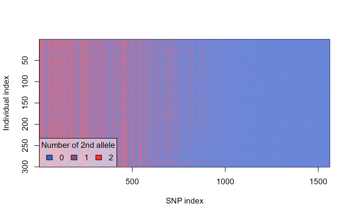 Note that the SNPs are ordered by their mutation id, which should
roughly correspond to their order of origination, so the leftmost
mutations are the oldest, the rightmost the youngest. Using a genlight
object we can calculate a lot of population genetics metrics easily
using the package
Note that the SNPs are ordered by their mutation id, which should
roughly correspond to their order of origination, so the leftmost
mutations are the oldest, the rightmost the youngest. Using a genlight
object we can calculate a lot of population genetics metrics easily
using the package dartR. Let’s calculate Fst for
example.
p_fst <- dartR::gl.fst.pop(inds, nboots = 1, verbose = 0)
p_fst
#>              p2         p3 p1
#> p2           NA         NA NA
#> p3 0.0005873432         NA NA
#> p1 0.0139928734 0.00888913 NA
So generally those Fst values are low, which we would expect since our populations are not experiencing differential selection and the effects of drift are counteracted by migration between the populations. Nevertheless the pairwise Fst’s measured here are inversely proportional to the overall strength of migration between the population in our simulation. We can see this like this:
## convert migration rates into pairwise matrix using igraph
library(igraph)
#>
#> Attaching package: 'igraph'
#> The following objects are masked from 'package:future':
#>
#>     %->%, %<-%
#> The following objects are masked from 'package:purrr':
#>
#>     compose, simplify
#> The following objects are masked from 'package:dplyr':
#>
#>     as_data_frame, groups, union
#> The following objects are masked from 'package:stats':
#>
#>     decompose, spectrum
#> The following object is masked from 'package:base':
#>
#>     union
overall_mig_rates <- disp_mat %>%
  as.data.frame() %>%
  igraph::graph_from_data_frame() %>%
  igraph::as.undirected(mode = "collapse", edge.attr.comb = "mean") %>%
  igraph::as_adjacency_matrix(type = "lower", attr = "V3", sparse = FALSE)

diag(overall_mig_rates) <- NA
overall_mig_rates[upper.tri(overall_mig_rates)] <- NA

p_fst
#>              p2         p3 p1
#> p2           NA         NA NA
#> p3 0.0005873432         NA NA
#> p1 0.0139928734 0.00888913 NA
overall_mig_rates
#>       1   2  3
#> 1    NA  NA NA
#> 2 0.055  NA NA
#> 3 0.225 0.1 NA

plot(as.vector(overall_mig_rates), as.vector(p_fst))
We can see generally the populations with the lowest migration rates
also has the highest pairwise Fst, suggesting population with low
migration have differentiated the most, which makes sense. In this
particular example, the Fst seems to reach a minimum soon after, such
that the two higher migration pairs don’t differ much in their pairwise
Fsts. This could be a result of stochasticity. if we really want to know
whether migration rate effects Fst under a simple neutral model of
evolution, we should run many simulations and look at the average
effect. slimr makes this easy to do using templating. Let’s
simplify this model a little to just look at two populations at a time,
and then set it up to run many times with different migration rates
between them. Ww can also vary population size as it seems like this
should be an important mediator of any effects, given it will effect the
relative strength of drift in the populations.
slim_script(
  slim_block(initialize(), {
    initializeMutationRate(2e-6);
    initializeMutationType("m1", 0.5, "f", 0.0);
    initializeGenomicElementType("g1", m1, 1.0);
    initializeGenomicElement(g1, 0, 99999);
    initializeRecombinationRate(1e-8);
  }),
  slim_block(1, {
    sim.addSubpop("p1", slimr_template("pop_size", default = 100));
    sim.addSubpop("p2", ..pop_size..);
    p1.setMigrationRates(p2, slimr_template("m", default = 0.1));
    p2.setMigrationRates(p1, ..m..);
  }),
  slim_block(10000, late(), {
    slimr_output(sim.outputFull(), "final_output");
  })
) -> script_3

script_3
#> <slimr_script[3]>
#> block_init:initialize() {
#> initializeMutationRate(2e-06);
#> initializeMutationType("m1", 0.5, "f", 0);
#> initializeGenomicElementType("g1", m1, 1);
#> initializeGenomicElement(g1, 0, 99999);
#> initializeRecombinationRate(1e-08);
#> }
#>
#> block_2:1 early() {
#> sim.addSubpop("p1", ..pop_size..);
#> sim.addSubpop("p2", ..pop_size..);
#> p1.setMigrationRates(p2, ..m..);
#> p2.setMigrationRates(p1, ..m..);
#> }
#>
#> block_3:10000 late() {
#> {sim.outputFull() -> final_output}
#> }
#> This slimr_script has templating in block(s) block_2 for
#> variables pop_size and m.So in the above script we now have a placemarker for a
pop_size and a m parameter. We specified this
using the slimr_template function directly inserted into
the SLiM code. We also demonstrate a trick to reduce typing. We only
have to use the slimr_template function once for a given
variable, subsequent references to the same variable can be specified
directly using the ..x.. notation. Now to generate a script
with the templated variables replaced with values of our choosing, we
use the slim_script_render function. Here is an
example:
example_script <- slim_script_render(script_3, template = list(pop_size = 50, m = 0.05))
example_script
#> <slimr_script[3]>
#> block_init:initialize() {
#> initializeMutationRate(2e-06);
#> initializeMutationType("m1", 0.5, "f", 0);
#> initializeGenomicElementType("g1", m1, 1);
#> initializeGenomicElement(g1, 0, 99999);
#> initializeRecombinationRate(1e-08);
#> }
#>
#> block_2:1 early() {
#> sim.addSubpop("p1", 50);
#> sim.addSubpop("p2", 50);
#> p1.setMigrationRates(p2, 0.05);
#> p2.setMigrationRates(p1, 0.05);
#> }
#>
#> block_3:10000 late() {
#> {sim.outputFull() -> final_output}
#> }We can also pass a data.frame to
slim_script_render which will allow us to generate many
scripts at once, let’s setup a large number of scripts to explore
different values of our two parameters.
n_reps <- 300

param_df <- data.frame(pop_size = sample(5:100, n_reps, replace = TRUE),
                                                         m = runif(n_reps, 0, 0.5))

script_list <- slim_script_render(script_3,
                                   template = param_df)

script_list
#> <slimr_script_coll[300]>
#> <1>
#>
#> block_init:initialize() {
#> initializeMutationRate(2e-06);
#> initializeMutationType("m1", 0.5, "f", 0);
#> initializeGenomicElementType("g1", m1, 1);
#> initializeGenomicElement(g1, 0, 99999);
#> initializeRecombinationRate(1e-08);
#> }
#>
#> block_2:1 early() {
#> sim.addSubpop("p1", 85);
#> sim.addSubpop("p2", 85);
#> p1.setMigrationRates(p2, 0.379254172206856);
#> p2.setMigrationRates(p1, 0.379254172206856);
#> }
#>
#> block_3:10000 late() {
#> {sim.outputFull() -> final_output}
#> }
#>
#> <2>
#>
#> block_init:initialize() {
#> initializeMutationRate(2e-06);
#> initializeMutationType("m1", 0.5, "f", 0);
#> initializeGenomicElementType("g1", m1, 1);
#> initializeGenomicElement(g1, 0, 99999);
#> initializeRecombinationRate(1e-08);
#> }
#>
#> block_2:1 early() {
#> sim.addSubpop("p1", 41);
#> sim.addSubpop("p2", 41);
#> p1.setMigrationRates(p2, 0.26800632593222);
#> p2.setMigrationRates(p1, 0.26800632593222);
#> }
#>
#> block_3:10000 late() {
#> {sim.outputFull() -> final_output}
#> }
#>
#> <3>
#>
#> block_init:initialize() {
#> initializeMutationRate(2e-06);
#> initializeMutationType("m1", 0.5, "f", 0);
#> initializeGenomicElementType("g1", m1, 1);
#> initializeGenomicElement(g1, 0, 99999);
#> initializeRecombinationRate(1e-08);
#> }
#>
#> block_2:1 early() {
#> sim.addSubpop("p1", 37);
#> sim.addSubpop("p2", 37);
#> p1.setMigrationRates(p2, 0.0882677737390622);
#> p2.setMigrationRates(p1, 0.0882677737390622);
#> }
#>
#> block_3:10000 late() {
#> {sim.outputFull() -> final_output}
#> }
#>
#>
#> <...>
#>
#> and 297 more.This function returns a slimr_script_coll object, or a
slimr script collection. We can now use slim_run on this
object, which will run every script in the collection, one after the
other, and collect the results. We can specify a
parallel = TRUE argument to run the scripts in parallel.
slimr uses the future package for
parallelization. This means that the user must specify a future
plan prior to running slim_run which will
setup the workers to be used by slimr. If you want to use
parallelization with slimr, we recommend you familiarize
yourself with the future package. If in doubt
future::plan(future::multisession) is the most general
purpose specification which should work well on all platforms (and is
the recommended plan by future for best stability of parallelization).
You must also ensure the future and furrr
packages are installed for this functionality to work. Let’s try running
these:
start_time <- Sys.time()
if(requireNamespace("furrr", quietly = TRUE)) {

  future::plan(future::multisession)

  all_results <- slim_run(script_list, parallel = TRUE, progress = TRUE, throw_error = TRUE)

}
Cool! First let’s check if all simulation completed without error:
Let’s extract all the genomic data into genlight objects so we can
easily calculate Fst. Since this might also take a little while we will
parallelize this extraction as well using furrr (since we
already set a future plan, and furrr uses
future under the hood). Just in case any simulations give
us trouble, we will wrap the extraction in try() so that
the whole thing doesn’t fail for one error.
all_gl <- furrr::future_map(all_results,
                     ~suppressWarnings(suppressMessages(try(slim_extract_genlight(.x, "final_output")))),
                     .progress = TRUE)
Any errors?
errored <- which(sapply(all_gl, function(x) class(x) == "try-error"))
errored
#> integer(0)

purrr::map(errored,
           ~all_results[[.x]]$output_data$data)
#> list()
We got ‘r length(errored)’ errors. Examining their data strings, we can see that they all essentially had no mutations, which is why we couldn’t construct a genlight object. Let’s just filter these out and continue with our analysis by calculating Fst.
if(length(errored) > 0) {
  all_gl <- all_gl[-errored]
}

all_fsts <- furrr::future_map_dbl(all_gl,
                                  ~ {
                                    ploidy(.x) <- 2
                                    dartR::gl.fst.pop(.x, nboots = 1, verbose = 0)[2, 1]
                                  },
                                  .progress = TRUE)
#> Registered S3 method overwritten by 'pegas':
#>   method      from
#>   print.amova ade4
#> Registered S3 method overwritten by 'GGally':
#>   method from
#>   +.gg   ggplot2
#> Registered S3 method overwritten by 'genetics':
#>   method      from
#>   [.haplotype pegas
#> Registered S3 method overwritten by 'pegas':
#>   method      from
#>   print.amova ade4
#> Registered S3 method overwritten by 'GGally':
#>   method from
#>   +.gg   ggplot2
#> Registered S3 method overwritten by 'genetics':
#>   method      from
#>   [.haplotype pegas
#> Registered S3 method overwritten by 'pegas':
#>   method      from
#>   print.amova ade4
#> Registered S3 method overwritten by 'GGally':
#>   method from
#>   +.gg   ggplot2
#> Registered S3 method overwritten by 'genetics':
#>   method      from
#>   [.haplotype pegas
#> Registered S3 method overwritten by 'pegas':
#>   method      from
#>   print.amova ade4
#> Registered S3 method overwritten by 'GGally':
#>   method from
#>   +.gg   ggplot2
#> Registered S3 method overwritten by 'genetics':
#>   method      from
#>   [.haplotype pegas
#> Registered S3 method overwritten by 'pegas':
#>   method      from
#>   print.amova ade4
#> Registered S3 method overwritten by 'GGally':
#>   method from
#>   +.gg   ggplot2
#> Registered S3 method overwritten by 'genetics':
#>   method      from
#>   [.haplotype pegas
#> Registered S3 method overwritten by 'pegas':
#>   method      from
#>   print.amova ade4
#> Registered S3 method overwritten by 'GGally':
#>   method from
#>   +.gg   ggplot2
#> Registered S3 method overwritten by 'genetics':
#>   method      from
#>   [.haplotype pegas
#> Registered S3 method overwritten by 'pegas':
#>   method      from
#>   print.amova ade4
#> Registered S3 method overwritten by 'GGally':
#>   method from
#>   +.gg   ggplot2
#> Registered S3 method overwritten by 'genetics':
#>   method      from
#>   [.haplotype pegas
#> Registered S3 method overwritten by 'pegas':
#>   method      from
#>   print.amova ade4
#> Registered S3 method overwritten by 'GGally':
#>   method from
#>   +.gg   ggplot2
#> Registered S3 method overwritten by 'genetics':
#>   method      from
#>   [.haplotype pegas

end_time <- Sys.time()

end_time - start_time
#> Time difference of 3.607884 mins

cat("Total Duration:", end_time - start_time)
#> Total Duration: 3.607884
Firstly, negative values of Fst are incorrect, and usually reflect numerical inaccuracy around zero, so we will set negative Fst values to zero. Then let’s look at the distribution.
all_fsts[all_fsts < 0] <- 0.0
hist(all_fsts, breaks = 100)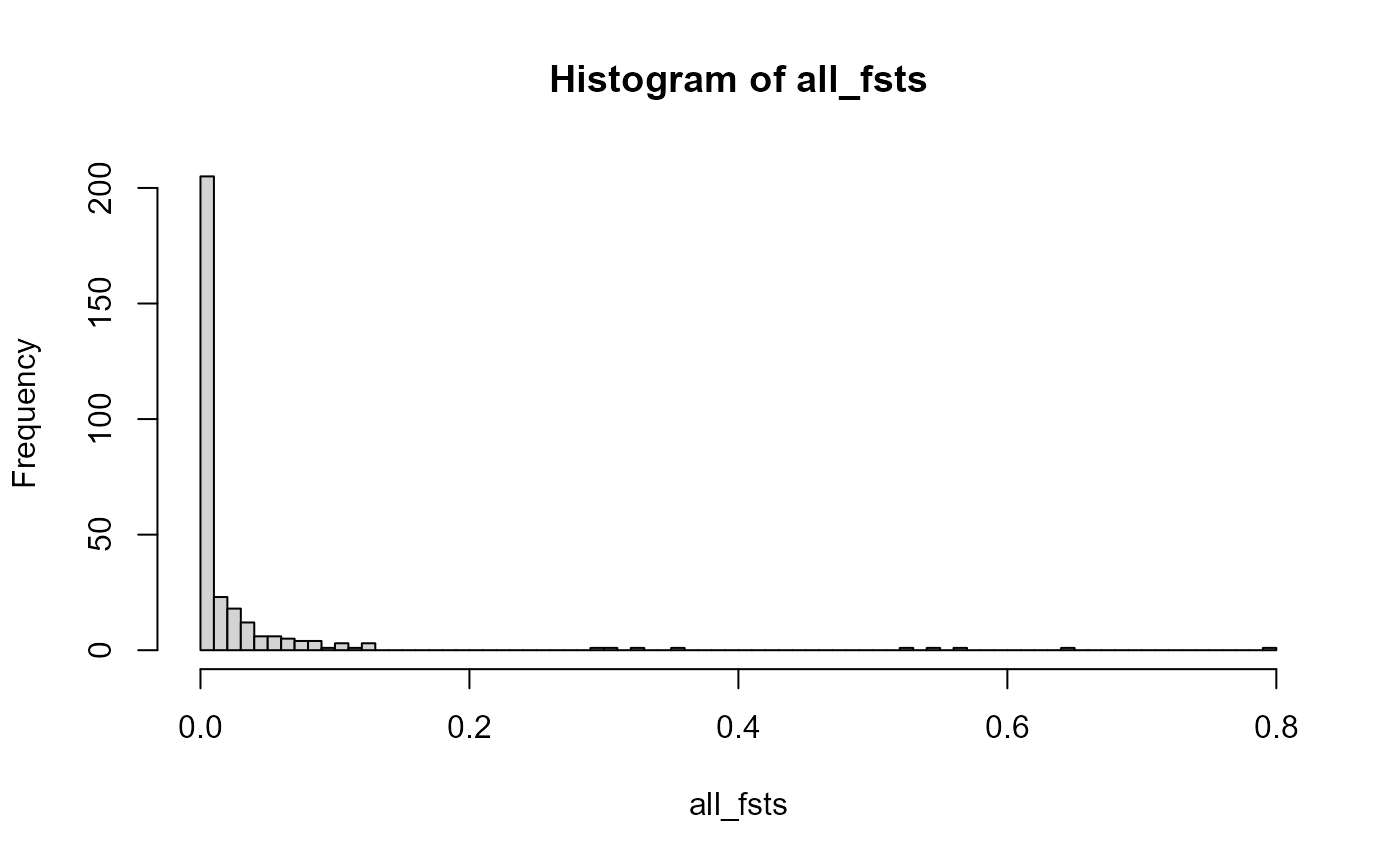 So how is Fst related to migration rate and population size? We can get
an idea by running a simple linear model. Then we will do plots.
So how is Fst related to migration rate and population size? We can get
an idea by running a simple linear model. Then we will do plots.
if(length(errored) > 0) {
  param_df <- param_df[-errored, ]
}

fst_dat <- param_df %>%
  dplyr::mutate(fst = all_fsts,
                pop_size_st = (pop_size - mean(pop_size)) / sd(pop_size),
                m_st = (m - mean(m)) / sd(m))

mod <- lm(fst ~ pop_size_st*m_st, data = fst_dat)
summary(mod)
#>
#> Call:
#> lm(formula = fst ~ pop_size_st * m_st, data = fst_dat)
#>
#> Residuals:
#>      Min       1Q   Median       3Q      Max
#> -0.08586 -0.03346 -0.00904  0.01365  0.68873
#>
#> Coefficients:
#>                   Estimate Std. Error t value Pr(>|t|)
#> (Intercept)       0.027855   0.004770   5.840 1.37e-08 ***
#> pop_size_st      -0.009437   0.004801  -1.966   0.0503 .
#> m_st             -0.031573   0.004802  -6.575 2.20e-10 ***
#> pop_size_st:m_st  0.005747   0.004712   1.220   0.2236
#> ---
#> Signif. codes:  0 '***' 0.001 '**' 0.01 '*' 0.05 '.' 0.1 ' ' 1
#>
#> Residual standard error: 0.08261 on 296 degrees of freedom
#> Multiple R-squared:  0.1391, Adjusted R-squared:  0.1304
#> F-statistic: 15.95 on 3 and 296 DF,  p-value: 1.231e-09
So both migration rate
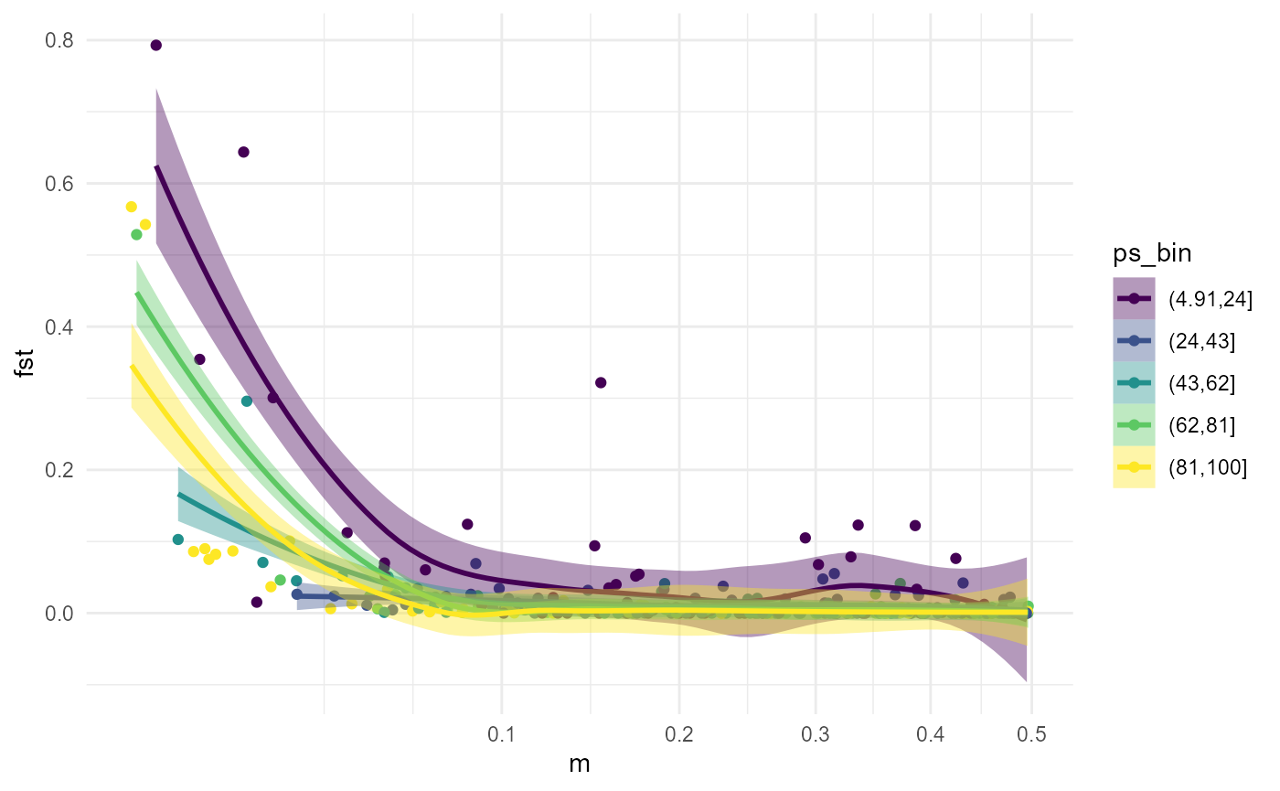
We can demonstrate the interaction by splitting our data into population size bins and plotting the migration rate relationship as separate lines for each bin.
fst_dat <- fst_dat %>%
  dplyr::mutate(ps_bin = cut(pop_size, 5, ordered_result = TRUE))

ggplot(fst_dat, aes(m, fst)) +
  geom_point(aes(colour = ps_bin)) +
  geom_smooth(aes(colour = ps_bin, fill = ps_bin)) +
  scale_x_sqrt() +
  theme_minimal()